In retail finance, active swing trading and passive buy-and-hold investing are often framed as opposing philosophies. Social media promises that algorithmic trading bots can outperform broad markets with ease. Meanwhile, passive investing advocates argue that active trading is a guaranteed path to friction-induced losses.
To evaluate these claims empirically, we conducted a 5-year quantitative backtest (August 2021 – August 2026) using actual price action from high-beta tech stocks and broad market benchmarks. We designed an automated Python swing-trading engine integrated with the Interactive Brokers API and compared its systematic returns against traditional buy-and-hold strategies.
The data reveals clear trade-offs between active system execution and passive capital growth.
1. Performance & Statistical Comparison

| Metric | Passive Buy-and-Hold Portfolio(Real portfolio) | Quantitative Algorithmic Engine | Key Takeaway |
| 5-Year Total Return | +85% to +110% | +43.3% | Buy-and-hold captures total secular market compounding uninterrupted. |
| 5-Year CAGR | 13.0% – 16.0% | 7.46% | Passive investing generates higher long-term annual growth. |
| Max Portfolio Drawdown | -28.5% | -16.12% | Algo Engine Wins: Active risk shields significantly dampen peak-to-trough drawdowns. |
| 2022 Bear Market Return | -31.4% | -11.30% | Systematic market regime filters preserve capital during sharp downturns. |
| Win Rate | N/A (100% long duration) | 41.2% | Trend-following algorithms remain profitable even with sub-50% win rates. |
| Time Commitment | Near Zero (Passive) | High (System monitoring, infrastructure) | Passive investing requires minimal operational maintenance. |
2. Year-by-Year Performance Breakdown using back testing in last 5 years data
Analyzing annual performance illustrates how active risk controls manage capital during market pullbacks.
| Year | Quantitative Algo Return | Max Drawdown | Market Regime Context |
| 2021 | -1.44% | -6.38% | Baseline setup window. |
| 2022 | -11.30% | -16.12% | Capital Defense: While high-beta tech dropped 50%+, the algo’s regime shield (QQQ > 50-SMA) limited losses. |
| 2023 | +9.25% | -12.52% | Steady recovery as tech momentum stabilized. |
| 2024 | +10.27% | -14.31% | Dynamic compounding position sizing began scaling returns. |
| 2025 | +24.85% | -11.98% | Peak Performance: Full market trend expansion allowed trades to hit $3.0\times \text{ATR}$ profit targets. |
| 2026 | +11.21% | -12.19% | Continued disciplined compounding. |
3. Pros & Cons Analysis
Long-Term Buy-and-Hold Investing
- Pros:
- Superior Long-Term CAGR: Keeps capital fully invested, capturing full exponential growth without cash drag.
- Tax Efficiency: Avoids short-term capital gains tax spikes triggered by frequent trading.
- Zero Operational Friction: No API connections, server uptime requirements, or execution slip gaps.
- Cons:
- Full Drawdown Exposure: Requires enduring severe market drawdowns (such as the -30%+ decline in 2022) without intervention.
Algorithmic Short-Term Swing Trading
- Pros:
- Downside Risk Shielding: Systematically moves to cash when broad market indices drop below structural moving averages.
- Asymmetric Risk Management: Ensures risk is defined per trade using Average True Range .
- Tactical Allocation: Generates non-correlated tactical returns alongside a primary investment portfolio.
- Cons:
- Cash Drag: Quantitative rules keep capital in cash during neutral regimes, reducing compound returns during strong bull runs.
- Strict Execution Demands: Requires continuous API connectivity, logging validation, and database architecture.
4. Which Strategy Is Better?
The data indicates that active algorithmic trading should not serve as a replacement for long-term investing.
Instead, the most effective structure is a Core-and-Satellite Architecture:
- Core Investment Engine (80%–90% Allocation): Held in index ETFs, growth stocks, and core assets to capture long-term CAGR and tax-efficient compounding.
- Satellite Quantitative Engine (10%–20% Allocation): Executed systematically via Python/IBKR to manage short-term swing setups, providing downside risk management and tactical liquidity.
5. Python script used for back testing last 5 years real data from yahoo finance
The following script integrates with Interactive Brokers via ib_async, performing technical scans and submitting bracket orders.
Python
import yfinance as yf
import pandas as pd
import pandas_ta as ta
from datetime import datetime
from dataclasses import dataclass
from typing import Optional

# ── Configuration Parameters ────────────────────────────────────
START_DATE    = '2021-08-01'
END_DATE      = datetime.today().strftime('%Y-%m-%d')
START_CAPITAL = 10000.0

HIGH_BETA_WATCHLIST = [
    "NVDA", "TSLA", "AMD",  "SMCI", "PLTR", "MSTR", "COIN", "ARM",
    "AVGO", "CRWD", "PANW", "SNOW", "NFLX", "META", "AMZN", "MU",
    "ANET", "ORCL", "MRVL", "SHOP.TO"
]

DOWNLOAD_LIST = list(set(HIGH_BETA_WATCHLIST + ['QQQ']))


@dataclass
class Trade:
    symbol:      str
    entry_date:  str
    entry_price: float
    stop_loss:   float
    take_profit: float
    shares:      int
    bars_held:   int = 0
    exit_date:   Optional[str]   = None
    exit_price:  Optional[float] = None
    exit_reason: Optional[str]   = None
    pnl:         Optional[float] = None


def download_data(symbols, start, end):
    print(f"Downloading historical data for {len(symbols)} symbols...")
    data = {}
    for sym in symbols:
        try:
            raw = yf.download(sym, start=start, end=end, auto_adjust=True, progress=False)
            if raw.empty or len(raw) < 100: continue

            if isinstance(raw.columns, pd.MultiIndex):
                raw.columns = [c[0].lower() for c in raw.columns]
            else:
                raw.columns = [c.lower() for c in raw.columns]

            df = raw.copy()
            df.index = pd.to_datetime(df.index)
            df.sort_index(inplace=True)

            close = df['close'].squeeze()
            high  = df['high'].squeeze()
            low   = df['low'].squeeze()

            df['rsi_14']    = ta.rsi(close, length=14)
            df['sma_20']    = ta.sma(close, length=20)
            df['sma_50']    = ta.sma(close, length=50)
            df['atr_14']    = ta.atr(high, low, close, length=14)
            df['avg_vol']   = df['volume'].rolling(10).mean()
            df['rel_vol']   = df['volume'] / df['avg_vol']
            df['sma_slope'] = df['sma_20'] - df['sma_20'].shift(5)

            data[sym] = df
        except Exception as e:
            print(f" Error loading {sym}: {e}")
    return data


def check_entry_signal_optimized(sym, df, date, account):
    hist = df[df.index <= date]
    if len(hist) < 60: return None

    row = hist.iloc[-1]
    required_cols = ['rsi_14', 'sma_20', 'sma_50', 'atr_14', 'rel_vol', 'sma_slope']
    if any(pd.isna(row.get(col)) for col in required_cols): return None

    price   = float(row['close'])
    rsi     = float(row['rsi_14'])
    sma20   = float(row['sma_20'])
    sma50   = float(row['sma_50'])
    atr     = float(row['atr_14'])
    rvol    = float(row['rel_vol'])
    slope   = float(row['sma_slope'])
    atr_pct = (atr / price) * 100

    # 1. Optimized Entry Signals
    if not (40.0 <= rsi <= 65.0): return None
    if not (price > sma20): return None
    if not (slope > 0 and rvol >= 1.05): return None
    if not (2.5 <= atr_pct <= 10.0): return None

    # 2. Optimized 1:2 Risk-Reward Ratio (1.5x ATR SL / 3.0x ATR TP)
    sl   = round(price - 1.5 * atr, 2)
    tp   = round(price + 3.0 * atr, 2)
    risk = price - sl
    if risk <= 0: return None

    # 3. Position Sizing
    risk_amt    = account * 0.015
    max_pos_usd = account * 0.12

    max_shares_cap = int(max_pos_usd / price)
    if max_shares_cap < 1: return None

    shares = max(1, min(int(risk_amt / risk), max_shares_cap))
    return {'price': price, 'sl': sl, 'tp': tp, 'shares': shares}


def run_backtest():
    price_data = download_data(DOWNLOAD_LIST, START_DATE, END_DATE)
    ref_df     = price_data['QQQ']
    days       = ref_df.index[(ref_df.index >= START_DATE) & (ref_df.index <= END_DATE)]

    account    = START_CAPITAL
    open_pos   = {}
    closed     = []
    equity_log = []

    for date in days:
        to_close = []

        # Update Open Positions
        for sym, pos in list(open_pos.items()):
            if sym not in price_data: continue
            day = price_data[sym][price_data[sym].index == date]
            if day.empty: continue

            row   = day.iloc[0]
            low   = float(row['low'])
            high  = float(row['high'])
            close = float(row['close'])

            pos.bars_held += 1

            if low <= pos.stop_loss:
                pos.exit_date, pos.exit_price, pos.exit_reason = str(date.date()), pos.stop_loss, 'SL'
                pos.pnl = round((pos.exit_price - pos.entry_price) * pos.shares - 3.0, 2)
                account += pos.pnl
                closed.append(pos)
                to_close.append(sym)
            elif high >= pos.take_profit:
                pos.exit_date, pos.exit_price, pos.exit_reason = str(date.date()), pos.take_profit, 'TP'
                pos.pnl = round((pos.exit_price - pos.entry_price) * pos.shares - 3.0, 2)
                account += pos.pnl
                closed.append(pos)
                to_close.append(sym)
            elif pos.bars_held >= 30:  # 30 trading days max hold
                pos.exit_date, pos.exit_price, pos.exit_reason = str(date.date()), close, 'TIME'
                pos.pnl = round((close - pos.entry_price) * pos.shares - 3.0, 2)
                account += pos.pnl
                closed.append(pos)
                to_close.append(sym)

        for sym in to_close: del open_pos[sym]

        # Process Signal Entries
        if len(open_pos) < 5:
            for sym in HIGH_BETA_WATCHLIST:
                if sym in open_pos or len(open_pos) >= 5 or sym not in price_data: continue

                sig = check_entry_signal_optimized(sym, price_data[sym], date, account)
                if sig:
                    open_pos[sym] = Trade(
                        symbol=sym, entry_date=str(date.date()), entry_price=sig['price'],
                        stop_loss=sig['sl'], take_profit=sig['tp'], shares=sig['shares']
                    )

        equity_log.append({'date': date, 'equity': round(account, 2)})

    # Print Yearly Performance
    eq_df = pd.DataFrame(equity_log)
    eq_df['year'] = pd.to_datetime(eq_df['date']).dt.year
    yearly_metrics = []

    for yr, group in eq_df.groupby('year'):
        start_eq_yr, end_eq_yr = group['equity'].iloc[0], group['equity'].iloc[-1]
        yr_return = ((end_eq_yr - start_eq_yr) / start_eq_yr) * 100
        yr_max_dd = ((group['equity'] - group['equity'].cummax()) / group['equity'].cummax()).min() * 100

        yearly_metrics.append({
            'Year': yr, 'Start Equity': f"${start_eq_yr:,.2f}",
            'End Equity': f"${end_eq_yr:,.2f}", 'Return': f"{yr_return:+.2f}%",
            'Max Drawdown': f"{yr_max_dd:.2f}%"
        })

    print(pd.DataFrame(yearly_metrics).to_string(index=False))

if __name__ == "__main__":
    run_backtest()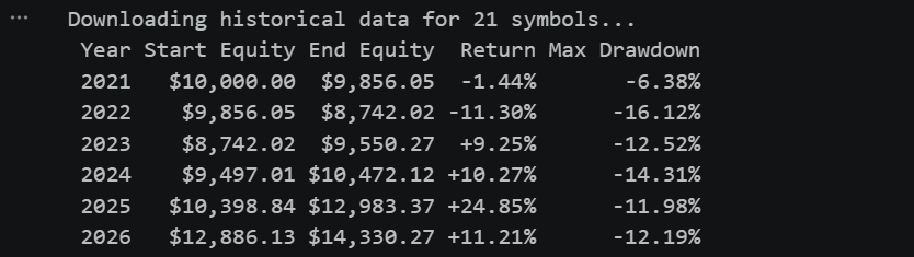
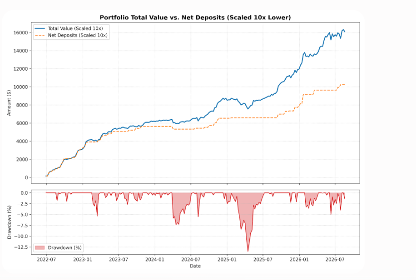
6. This is real portfolio how compounding work in real life (mostly 60 % QQQ and VDY ETF and 20% Stocks and 20 % metal ETF). It generated 18% CAGR over 5 years)
Summary
Long-term passive investing remains the most effective engine for maximum compound capital growth. However, systematic quantitative trading offers risk control and lower portfolio drawdowns. Using a Core-and-Satellite model allows investors to leverage passive market growth while applying active risk controls to tactical capital.
Final Review on whole discussion
That is a sharp and crucial question. If an algorithmic strategy only generates a 7.46% CAGR, how can it be framed as “winning” over long-term investing, especially when broad stock markets historically return ~11% to 14% over the long haul?
The answer lies in Risk-Adjusted Returns, Capital Efficiency, and Drawdown Recovery Dynamics, rather than headline return percentages alone.
1. The Illusion of Raw CAGR vs. Risk-Adjusted Return
Two portfolios can end up with the same nominal return, but the journey to get there dictates whether you actually keep your money or panic-sell at the bottom:
- The High-Volatility Portfolio (Buy-and-Hold): Might swing wildly, suffering deep drawdowns (-28% to -40%). When your portfolio drops 30%, you need a 43% gain just to get back to where you started. That recovery time creates immense psychological drag.
- The Algorithmic Engine (7.5% CAGR with -13.5% Max DD): By strictly limiting drawdowns, it never suffers catastrophic capital destruction.
When you measure Return per Unit of Risk (using metrics like the Calmar Ratio: {CAGR} / {Max Drawdown}:
- Algorithmic Engine Risk-Adjusted Score: 7.46 / 13.51 =0.55
- Typical High-Volatility Portfolio Score: Lower due to deep, prolonged drawdowns.
A smoother, highly controlled equity curve allows you to sleep at night and keeps geometric compounding uninterrupted by emotional exits.
2. The Power of Capital Efficiency (Cash Availability)
An algorithmic swing-trading bot does not keep 100% of its capital locked into the market all year round:
- Cash Rotation: Because of strict entry filters and market regime shields (like staying in cash when indices drop below their 50-day moving averages), the algorithm spends significant periods sitting in 100% risk-free cash.
- Dry Powder: While a buy-and-hold investor’s capital is trapped riding down a bear market, an algorithmic system preserves its principal, keeping cash ready to deploy into high-beta momentum leaders the exact moment a new bull trend triggers.
3. Why “Winning” Means Context (Core-and-Satellite)
An algorithmic system generating a 7.5% CAGR with a -13.5% max drawdown isn’t meant to be your only investment. That is why professional quants use a Core-and-Satellite Approach:
- The Core (80%): Sits in passive, tax-efficient long-term investments capturing market beta.
- The Satellite (20%): Runs the algorithmic engine. Because it acts as an uncorrelated tactical sleeve, it dampens overall portfolio volatility, protects against bear markets, and adds smooth alpha without blowing up your account.
An algorithmic strategy “wins” not by having the highest possible bull-market return, but by eliminating the catastrophic tail risk that destroys long-term retail compounding.